Lesson Contents
Introduction
This blog post details how to physically “draw” the OSPF topology within an area using on the “show ip ospf database” command hierarchy. As a disclaimer, this is an advanced topic, and it assumes you already have knowledge on the LSA types and their uses. As a prerequisite for this lesson, please read the below blog post from Cisco’s website that details how the read the OSPF LSDB and even touches on how to draw topologies based on it.
Reading and Understanding the OSPF Database
This blog post is meant to add some detail to the existing post. First, we need to discuss some basics of “graph theory”.
Graph Theory Basics
The word “graph” is commonly used to describe OSPF data structures because under the hood, OSPF uses the concept of a mathematical graph. I will spare you the textbook definitions and use some simplistic terminology:
- Graphs consist of edges and vertices.
- Vertices are nodes in the graph and contain names. In OSPF, this is the RID.
- Edges connect exactly TWO vertices together. In OSPF, these edges are typically the links (or subnets) between routers. You may be wondering how a multi-access network can exist with this restriction. I will answer this question shortly.
- Graphs may be weighted or non-weighted. A non-weighted graph would contain edges that are all considered equal in weight for the SPF algorithm. We know that this weight is represented by OSPF cost and is adjustable, so OSPF relies on a “weighted” graph.
- Graphs may be directed or non-directed. A non-directed graph means that a path can exist in either direction transiting an edge between two vertices. A directed graph relies on explicitly specifying which way paths may exist. A directed graph is analogous to a one-way street, while a non-directed graph is analogous to a two way street. OSPF, however, uses a directed graph; although the link between vertices is only represented once, recall that we can set the cost differently on either end of the link. The underlying directed graph allows us to do this, possibly causing asymmetric paths in our network. Thus, every link is OSPF is actually a composition of two “one-way” streets, if you will, both with adjustable costs. This becomes important for multi-access networks.
Understanding OSPF graph components
The required reading from Cisco’s website included mapping out many other types of LSAs which are not directly relevant to the construction of the OSPF graph within an area. Only LSA-1 and LSA-2 are used to actually build the graph since the OSPF area is the definition of the OSPF link-state domain. Inter-area and external routes rely on distance-vector-style behavior for computation. Recall that routers in an area sum the cost to the ABR or ASBR* (based on the intra-area graph) with the advertised metric contained within the LSA-3 or LSA-4, depending on the situation. I do not cover this procedure as it is already very well documented.
*I will offer one small comment with respect to the path-cost algorithm for LSA-5. If the forward address is 0.0.0.0, the the cost used to reach the ASBR is used in the total path-cost. If the FA is anything else, the cost to the FA is used. This is beyond the scope of this blog post, and I do not discuss this further.
Every router represents a vertex in our graph. Within an LSA-1 you will find one of four different connection types:
- Transit network: This link type indicates a connection to a DR. Notice that the network mask information is not present here, and also that the addresses here are the interface addresses, not the RIDs. This is important.
- Point-to-point: This link type indicates a connection to exactly one other router. This is more of a classic “edge” that first comes to mind when one thinks about graph theory. This link type DOES NOT contain any routing information and is used only for OSPF graph construction.
- Stub network: Often times, this is a link type that has no neighbors. This is useful for representing a subnet, such as a loopback or user LAN. You will also see stub networks to represent the subnets for point-to-point links in many cases by default. We will explore how to disable this feature later.
- Virtual link: Like a point-to-point link, a virtual link connects exactly two routers. There is no associated routing information with this link.
Mapping links to subnets is not as simple. Consider a multi-access OSPF network with four routers on the segment. Assuming default configuration, there would be one DR, one BDR, and two DRothers. Most people know that “everyone forms an adjacency with the DR and BDR, but DRothers do not form adjacencies with one another”. This is true. So, would our graph look like this?
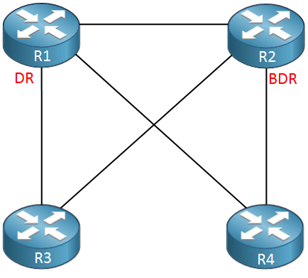
No, it would not. First of all, how would you assign costs in this way? This graph implies that traffic must physically transit the DR or BDR, which we know does not happen. Also, this seems like an awful lot of edges for such a simple topology.
Do you remember the word “pseudonode” from your OSPF studies? The aforementioned Cisco post glazes over this detail in their drawings a little bit. When a router wins the DR election, it does not become the DR, but rather earns the right to maintain the DR’s pseudonode. Remember our graph theory restriction: An edge connects exactly TWO vertices. This pseudonode is a vertex in the graph and serves as an interface to which all other routers on the segment connect. But what about the BDR? While it is subscribed to the All-DR multicast group of 224.0.0.6 (thus hearing everyone the DR does), it DOES NOT play a role in the OSPF graph. It is loosely analogous to HSRP standby routers where its role is one of remaining a “hot standby”.
Key point: The router we casually say is the DR is not really the DR. When this router does its local OSPF computation, it also has to consult the “DR” (which is locally stored) to find out the RIDs of other routers on the segment. We will see this in action soon.
This pseudonode is represented by the LSA-2 that maintains a connection to every router on the segment. As mentioned earlier, this LSA-2 maintains the network mask for the segment as individual LSA-1s do not store this information. The only link type within an LSA-1 that contains network mask information is the stub network, which is specifically used to create intra-area, or “O” routes in the routing table for all non-multi-access networks.
Drawing the graph
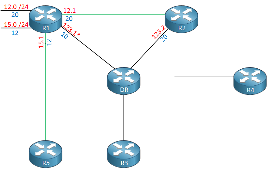
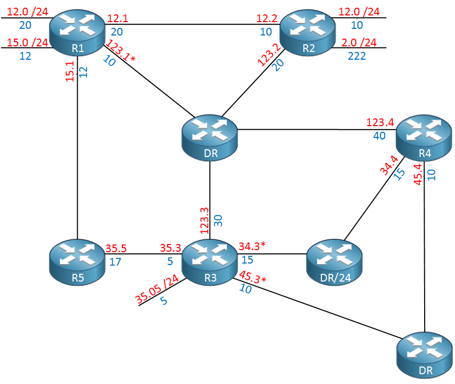
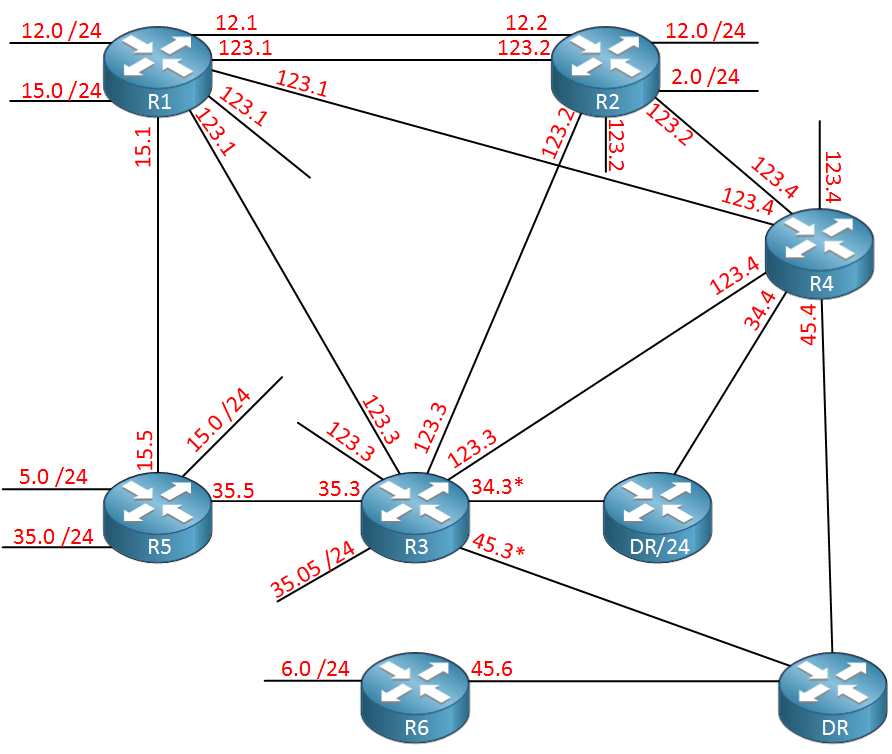
Enough talk. Let’s check out our topology and hit the command line. As an administrative note, additions to the graph at each step are shown in green.
We should immediately identify the basic characteristics of this topology:
- We have 6 routers with all interfaces contained within area 0, which means we should have 6 LSA-1s.
- We have 3 multi-access networks (not counting the neighborless LANs), which means we should have 3 LSA-2s.
- We should have a total of 9 vertices in the graph (sum of LSA1 and LSA2).
A quick verification of these facts is achieved using simply “show ip ospf database database-summary”. Alternatively, you could issue the “show ip ospf database” command simply count lines, but this method is time consuming and error prone, especially with large OSPF areas.
All routers in the topology will agree on this topology and compute their own shortest paths to all remote OSPF destinations for which routing information is available within the LSAs. For the purpose of this exercise, we will draw the graph beginning with R1, but using any router is acceptable.
First, R1 examines it’s own LSA-1 to see its local links and also to which other routers it is connected. You can use one of three commands to see you own LSA-1:
- show ip ospf database router self-originate
- show ip ospf database router 1.1.1.1
- show ip ospf database router adv-router 1.1.1.1
The reason the last two commands are interchangeable in this case is because LSA-1s always have the Link ID field equal to the RID field. Thus, you may query the database using either criterion. Normally, however, using the “adv-router” field for other LSAs can yield extraneous output as all LSAs originated from that RID are displayed. The Link ID method is often preferred because it is more specific.
R1#show ip ospf database router self-originate

            OSPF Router with ID (1.1.1.1) (Process ID 1)

		Router Link States (Area 0)

  LS age: 1208
  Options: (No TOS-capability, DC)
  LS Type: Router Links
  Link State ID: 1.1.1.1
  Advertising Router: 1.1.1.1
  LS Seq Number: 80000004
  Checksum: 0x3EDA
  Length: 84
  Number of Links: 5

    Link connected to: a Transit Network
     (Link ID) Designated Router address: 10.0.123.1
     (Link Data) Router Interface address: 10.0.123.1
      Number of TOS metrics: 0
       TOS 0 Metrics: 10

    Link connected to: another Router (point-to-point)
     (Link ID) Neighboring Router ID: 5.5.5.5
     (Link Data) Router Interface address: 10.0.15.1
      Number of TOS metrics: 0
       TOS 0 Metrics: 12

    Link connected to: a Stub Network
     (Link ID) Network/subnet number: 10.0.15.0
     (Link Data) Network Mask: 255.255.255.0
      Number of TOS metrics: 0
       TOS 0 Metrics: 12

    Link connected to: another Router (point-to-point)
     (Link ID) Neighboring Router ID: 2.2.2.2
     (Link Data) Router Interface address: 10.0.12.1
      Number of TOS metrics: 0
       TOS 0 Metrics: 20

    Link connected to: a Stub Network
     (Link ID) Network/subnet number: 10.0.12.0
     (Link Data) Network Mask: 255.255.255.0
      Number of TOS metrics: 0
       TOS 0 Metrics: 20
We have a total of 5 “links”. Clearly our diagram only shows 3 links, though. Let’s see if we can account for the difference. Examining the output above, and comparing this against what we have learned so far in this blog, we can conclude the following:
- R1 is connected to exactly one multi-access network, and coincidentally, represents the DR for that network. Notice that I did not say “R1 is the DR”, because it is not. It performs the duties of the DR.
- R1 is connected to exactly two other routers via point-to-point connections. These links, combined with #1, make up for our 3 links in the diagram.
- R1 also has two stub networks, one to represent each of the point-to-point links shown above. Without these entries, other routers would not have routing information for the 10.0.15.0/24 and 10.0.12.0/24 subnets.
Let’s digest this information as follows. Notice how we get pretty much every piece of information from this output except the interface numbers. We can record the link costs (remember, the graph is directed, so these costs could differ on both sides) and interface IP addresses also.
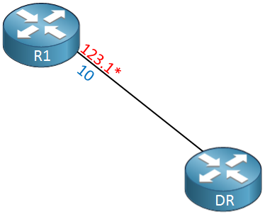
Where do we go next? What should we draw? For simplicity, let’s process them in order. R1 needs to ask the DR “What other routers do you know about?” We would expect to see our own RID in the DR’s roster, but at least one other one as well. Notice that we specify the Link ID here to be specific; I do not want to see all of R1’s self-originated LSAs, but rather a specific LSA.
R1#show ip ospf database network 10.0.123.1

            OSPF Router with ID (1.1.1.1) (Process ID 1)

		Net Link States (Area 0)

  Routing Bit Set on this LSA
  LS age: 4
  Options: (No TOS-capability, DC)
  LS Type: Network Links
  Link State ID: 10.0.123.1 (address of Designated Router)
  Advertising Router: 1.1.1.1
  LS Seq Number: 80000002
  Checksum: 0x4B33
  Length: 40
  Network Mask: /24
	Attached Router: 1.1.1.1
	Attached Router: 2.2.2.2
	Attached Router: 3.3.3.3
	Attached Router: 4.4.4.4
The DR for this segment says that 4 routers are attached. It also provides the network mask, but not much else. Let’s add this to our diagram. It is also interesting to note that despite being a vertex in our graph, the DR does not list any OSPF costs for these four connections. We will investigate this more later.
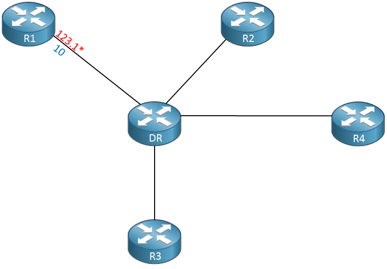
For the purpose of drawing the picture, you can go any way you like from this point.
- You can continue to process R1’s LSA-1 entries in any order you like.
- You can look at R2’s (2.2.2.2) LSA-1, since we now know about it.
- You can look at R3’s (3.3.3.3) LSA-1, since we now know about it.
- You can look at R3’s (4.4.4.4) LSA-1, since we now know about it.
Personally, I prefer to finish up one LSA-1 at a time, so I will select option #1. For the purpose of this tutorial, I am going to examine the next two entries in R1’s LSA-1 together. Here they are again:
Link connected to: another Router (point-to-point)
     (Link ID) Neighboring Router ID: 5.5.5.5
     (Link Data) Router Interface address: 10.0.15.1
      Number of TOS metrics: 0
       TOS 0 Metrics: 12

    Link connected to: a Stub Network
     (Link ID) Network/subnet number: 10.0.15.0
     (Link Data) Network Mask: 255.255.255.0
      Number of TOS metrics: 0
       TOS 0 Metrics: 12
The first one is straightforward; we have a direct link to R5 (5.5.5.5), so let’s draw that, along with the cost/IP information. This stub network is only for routing reachability, so let’s draw it exactly as the LSDB instructs; as a stub. I like to use an “X” at the end of the link to show that it is a stub network. Be sure to write down the network mask as it is not contained anywhere else, and other routers need to know it.
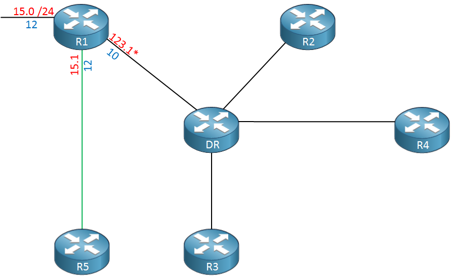
Let’s finish up R1’s LSA-1 entries. One more P2P link to R2 with corresponding stub network. At this point, we know everything R1 knows about the graph.

Currently, we have R2, R3, R4, and R5 as routers that R1 can see, but has no idea what their link states look like. I will continue with R2 for the purposes of sequencing. Let’s ask R2 what he is up to.
R1#show ip ospf database router 2.2.2.2
OSPF Router with ID (1.1.1.1) (Process ID 1)
Router Link States (Area 0)
LS age: 535
Options: (No TOS-capability, DC)
LS Type: Router Links
Link State ID: 2.2.2.2
Advertising Router: 2.2.2.2
LS Seq Number: 80000007
Checksum: 0xD9C2
Length: 72
Number of Links: 4
Link connected to: a Transit Network
(Link ID) Designated Router address: 10.0.123.1
(Link Data) Router Interface address: 10.0.123.2
Number of TOS metrics: 0
TOS 0 Metrics: 20
Link connected to: another Router (point-to-point)
(Link ID) Neighboring Router ID: 1.1.1.1
(Link Data) Router Interface address: 10.0.12.2
Number of TOS metrics: 0
TOS 0 Metrics: 10
Link connected to: a Stub Network
(Link ID) Network/subnet number: 10.0.12.0
(Link Data) Network Mask: 255.255.255.0
Number of TOS metrics: 0
TOS 0 Metrics: 10
Link connected to: a Stub Network
(Link ID) Network/subnet number: 10.0.2.0
(Link Data) Network Mask: 255.255.255.0
Number of TOS metrics: 0
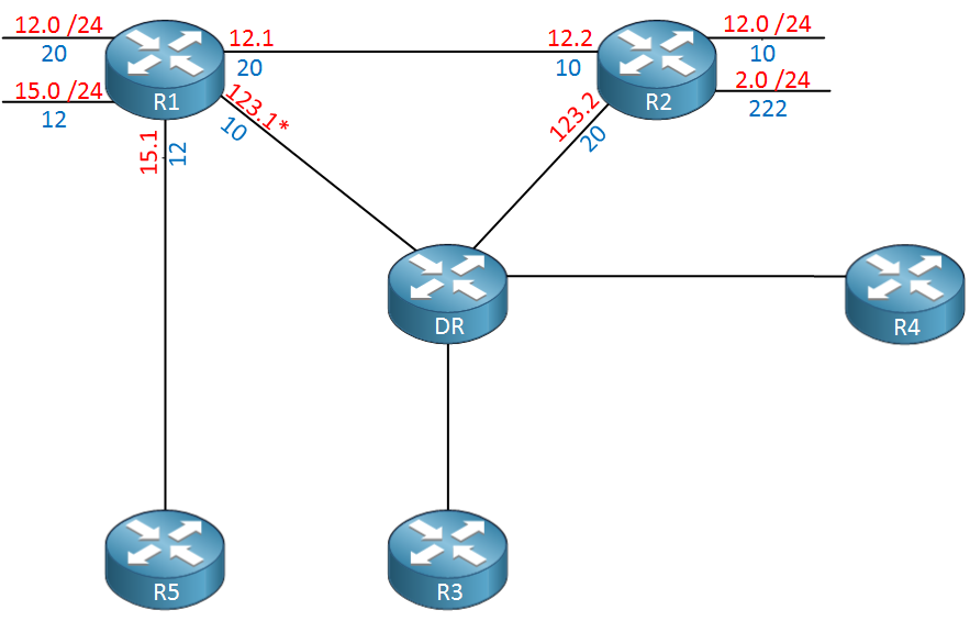
TOS 0 Metrics: 222First, R2 says it is connected to a DR represented by 10.0.123.1 (asterisk in diagram). That should look familiar, considering that is the method by which we discovered R2 in the first place. Let’s add R2’s interface and cost information to this link that we drew previously.
R2 also claims to be connected to R1 via a P2P link also, and as expected, contains a corresponding stub link with network mask information. Let’s draw these, always remembering our costs and network masks. We can quickly see that our costs are asymmetric!
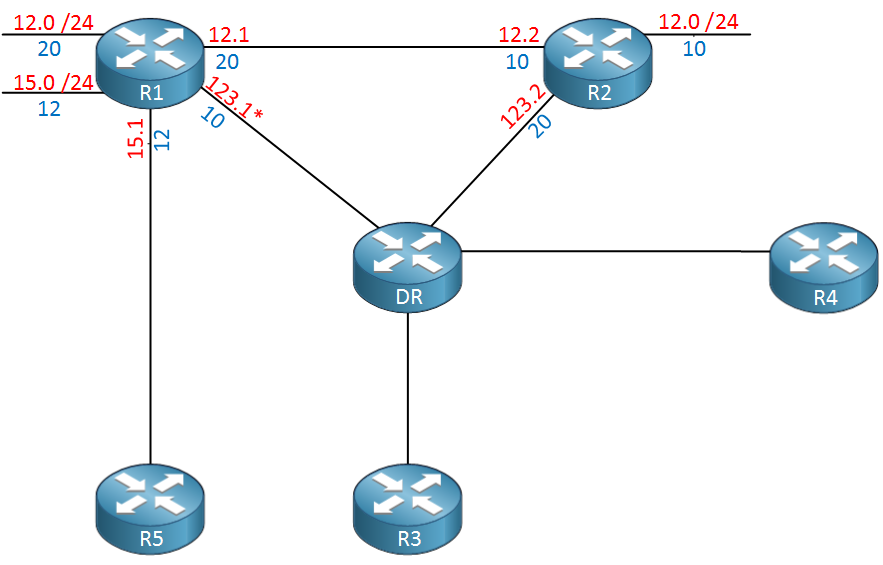
R2 also has a true “stub” user LAN. This interface is running network-type broadcast, but since there are no OSPF speakers on the segment, no LSA-2 is generated. Let’s draw this as we would draw any other stub network. R2 is now complete.
We will move more quickly through the remaining routers, showing all the CLI output and drawing all necessary information at once. R3 is next.
R1#show ip ospf database router 3.3.3.3

            OSPF Router with ID (1.1.1.1) (Process ID 1)

		Router Link States (Area 0)

  LS age: 784
  Options: (No TOS-capability, DC)
  LS Type: Router Links
  Link State ID: 3.3.3.3
  Advertising Router: 3.3.3.3
  LS Seq Number: 80000009
  Checksum: 0xD86A
  Length: 84
  Number of Links: 5

    Link connected to: a Transit Network
     (Link ID) Designated Router address: 10.0.45.3
     (Link Data) Router Interface address: 10.0.45.3
      Number of TOS metrics: 0
       TOS 0 Metrics: 10

    Link connected to: a Transit Network
     (Link ID) Designated Router address: 10.0.123.1
     (Link Data) Router Interface address: 10.0.123.3
      Number of TOS metrics: 0
       TOS 0 Metrics: 30

    Link connected to: another Router (point-to-point)
     (Link ID) Neighboring Router ID: 5.5.5.5
     (Link Data) Router Interface address: 10.0.35.3
      Number of TOS metrics: 0
       TOS 0 Metrics: 5

    Link connected to: a Stub Network
     (Link ID) Network/subnet number: 10.0.35.0
     (Link Data) Network Mask: 255.255.255.0
      Number of TOS metrics: 0
       TOS 0 Metrics: 5

    Link connected to: a Transit Network
     (Link ID) Designated Router address: 10.0.34.3
     (Link Data) Router Interface address: 10.0.34.3
      Number of TOS metrics: 0
       TOS 0 Metrics: 15
Looks like R3 is representing the DR for two new network segments (indicated with an asterisk as usual). We need to double-back and check those LSA-2s before we finish. In the meantime, we need to draw R3’s P2P link to R2 (and its corresponding stub network) and it’s links to three other DRs.
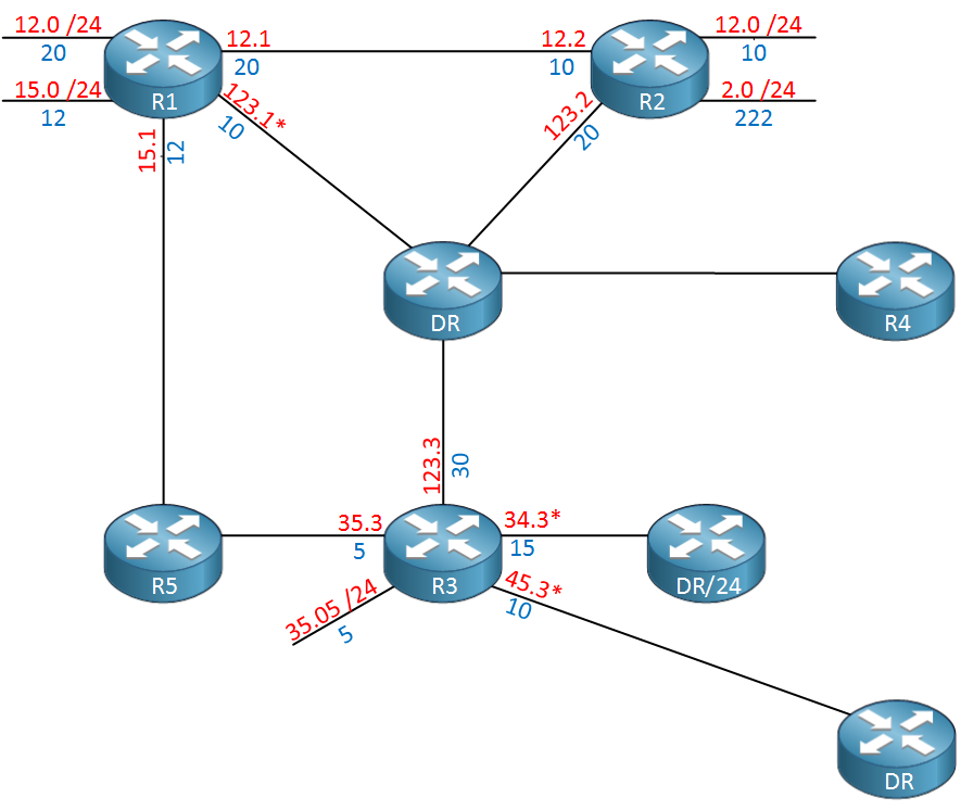
Next up is R4.
R1#show ip ospf database router 4.4.4.4

            OSPF Router with ID (1.1.1.1) (Process ID 1)

		Router Link States (Area 0)

  LS age: 834
  Options: (No TOS-capability, DC)
  LS Type: Router Links
  Link State ID: 4.4.4.4
  Advertising Router: 4.4.4.4
  LS Seq Number: 80000008
  Checksum: 0x695F
  Length: 60
  Number of Links: 3

    Link connected to: a Transit Network
     (Link ID) Designated Router address: 10.0.45.3
     (Link Data) Router Interface address: 10.0.45.4
      Number of TOS metrics: 0
       TOS 0 Metrics: 10

    Link connected to: a Transit Network
     (Link ID) Designated Router address: 10.0.123.1
     (Link Data) Router Interface address: 10.0.123.4
      Number of TOS metrics: 0
       TOS 0 Metrics: 40

    Link connected to: a Transit Network
     (Link ID) Designated Router address: 10.0.34.3
     (Link Data) Router Interface address: 10.0.34.4
      Number of TOS metrics: 0
       TOS 0 Metrics: 15
Our graph is coming together quickly. Looks like R3 and R4 both claim to be connected to a DR at 10.0.34.3. We should confirm this.
R1#show ip ospf database network 10.0.34.3

            OSPF Router with ID (1.1.1.1) (Process ID 1)

		Net Link States (Area 0)

  Routing Bit Set on this LSA
  LS age: 1275
  Options: (No TOS-capability, DC)
  LS Type: Network Links
  Link State ID: 10.0.34.3 (address of Designated Router)
  Advertising Router: 3.3.3.3
  LS Seq Number: 80000002
  Checksum: 0x5A87
  Length: 32
  Network Mask: /24
	Attached Router: 3.3.3.3
	Attached Router: 4.4.4.4
Just as we thought. Let’s record our results and examine R5 next.
R1#show ip ospf database router 5.5.5.5

            OSPF Router with ID (1.1.1.1) (Process ID 1)

		Router Link States (Area 0)

  LS age: 907
  Options: (No TOS-capability, DC)
  LS Type: Router Links
  Link State ID: 5.5.5.5
  Advertising Router: 5.5.5.5
  LS Seq Number: 80000005
  Checksum: 0xD8D9
  Length: 84
  Number of Links: 5

    Link connected to: another Router (point-to-point)
     (Link ID) Neighboring Router ID: 3.3.3.3
     (Link Data) Router Interface address: 10.0.35.5
      Number of TOS metrics: 0
       TOS 0 Metrics: 17

    Link connected to: a Stub Network
     (Link ID) Network/subnet number: 10.0.35.0
     (Link Data) Network Mask: 255.255.255.0
      Number of TOS metrics: 0
       TOS 0 Metrics: 17

    Link connected to: another Router (point-to-point)
     (Link ID) Neighboring Router ID: 1.1.1.1
     (Link Data) Router Interface address: 10.0.15.5
      Number of TOS metrics: 0
       TOS 0 Metrics: 17

    Link connected to: a Stub Network
     (Link ID) Network/subnet number: 10.0.15.0
     (Link Data) Network Mask: 255.255.255.0
      Number of TOS metrics: 0
       TOS 0 Metrics: 17

    Link connected to: a Stub Network
     (Link ID) Network/subnet number: 10.0.5.0
     (Link Data) Network Mask: 255.255.255.0
      Number of TOS metrics: 0
       TOS 0 Metrics: 30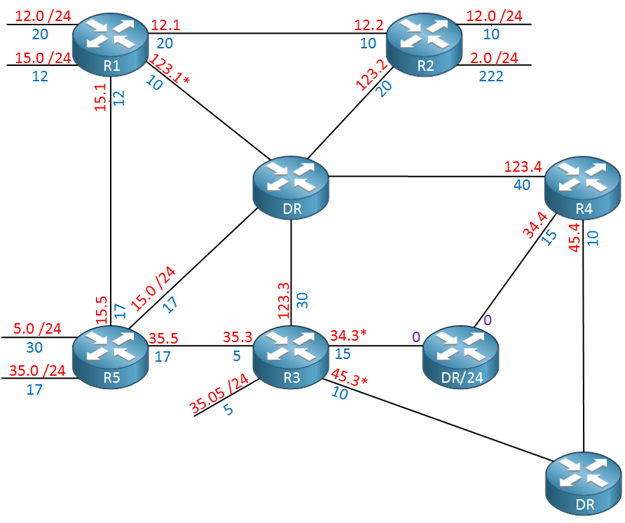
OK, that finishes up most of the topology. We seem to be missing R6 though. Why is that? Recall that R3 represents a third DR that we have not queried. Let’s see what that DR has to say.
R1#show ip ospf database network 10.0.45.3

            OSPF Router with ID (1.1.1.1) (Process ID 1)

		Net Link States (Area 0)

  Routing Bit Set on this LSA
  LS age: 1118
  Options: (No TOS-capability, DC)
  LS Type: Network Links
  Link State ID: 10.0.45.3 (address of Designated Router)
  Advertising Router: 3.3.3.3
  LS Seq Number: 80000003
  Checksum: 0x7445
  Length: 36
  Network Mask: /24
	Attached Router: 3.3.3.3
	Attached Router: 4.4.4.4
	Attached Router: 6.6.6.6
Looks like we found our sixth router. Let’s find out what its links look like.
R1#show ip ospf database router 6.6.6.6
OSPF Router with ID (1.1.1.1) (Process ID 1)
Router Link States (Area 0)
LS age: 1129
Options: (No TOS-capability, DC)
LS Type: Router Links
Link State ID: 6.6.6.6
Advertising Router: 6.6.6.6
LS Seq Number: 80000003
Checksum: 0x4822
Length: 48
Number of Links: 2
Link connected to: a Transit Network
(Link ID) Designated Router address: 10.0.45.3
(Link Data) Router Interface address: 10.0.45.6
Number of TOS metrics: 0
TOS 0 Metrics: 10
Link connected to: a Stub Network
(Link ID) Network/subnet number: 10.0.6.0
(Link Data) Network Mask: 255.255.255.0
Number of TOS metrics: 0
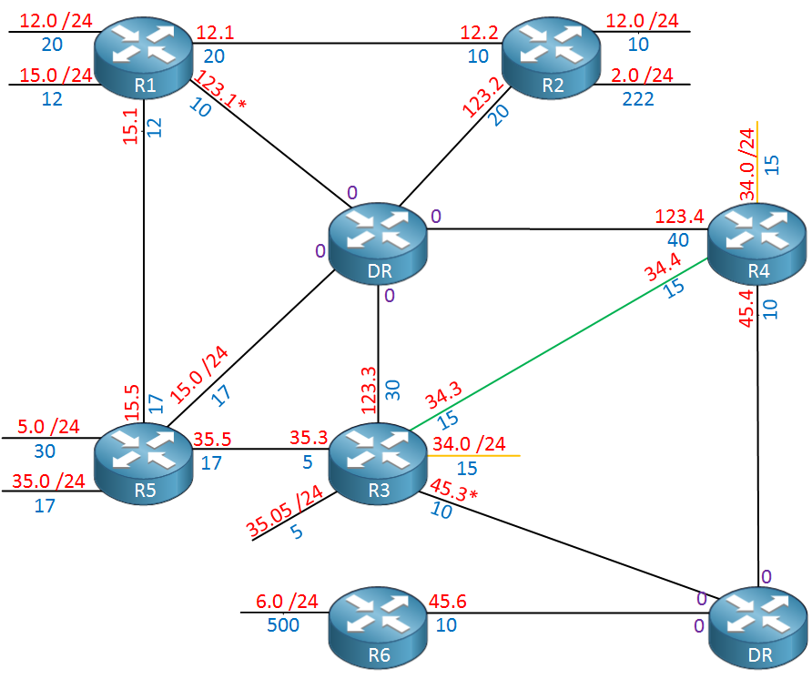
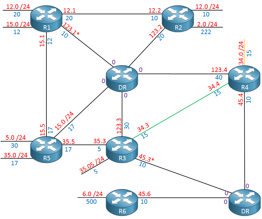
TOS 0 Metrics: 500OK, that is everything! Let’s look at the (almost) final graph.
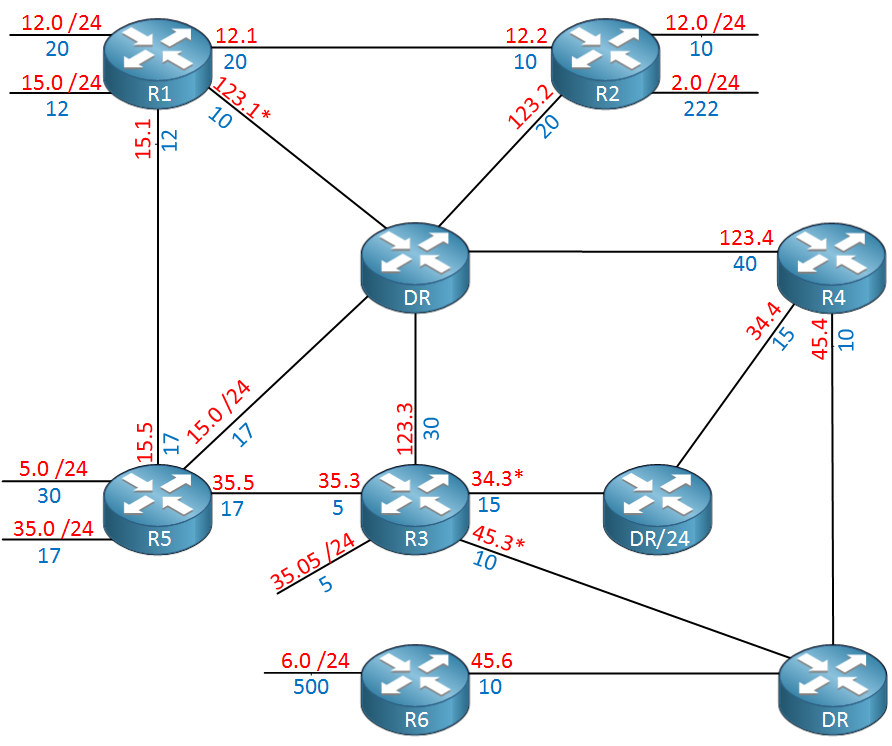
Before I identify what is missing, let’s draw some conclusions:
- The number of “lines” connected to a vertex must be equal to the “link count” expressed in the router’s LSA-1. Notice how R1 has 5 links. Remember how this confused us earlier? Now we have a quick sanity check for our drawing.
- Every edge connects exactly TWO vertices. Do you understand the significance of the mysterious “pseudonode” now?
- The DR on the link between R3 and R4 (10.0.34.0/24 link) doesn’t appear to be doing much. This is why it is common to see links connecting exactly two routers to be configured as “point-to-point” network type. We can reduce OSPF overhead by removing an entire vertex from the graph at no cost to us. In fact, it actually improves OSPF performance slightly, which we will discuss later.
We have a problem, though. Every vertex has an OSPF cost associated with each of its links except our DRs. Well, they are vertices in the graph, and they have to play by the rules. Think for a moment on what the costs of those DR links should be. Imagine that R4 is trying to route traffic to R6’s 10.0.6.0/24 subnet.
The cost would be 10 + 500, or 510. According to our graph, though, we transited our DR, yet no cost was incurred. The cost of the DR’s links is always zero, and it is the only vertex in the graph that can have zero-cost links. The entire purpose of the DR was not meant to be “another hop” or “another router”, but just to minimize adjacencies over a large shared segment. So, in reality, it isn’t really participating in routing per se, but from a purely theoretical perspective, its link-costs are zero.
The SPF algorithm still treats the DR as a vertex and as such must account for its link costs. As we know, when it comes to routing information, the DR is transparent. Let’s fill in those new costs and make our final graph (shown in purple for clarity).
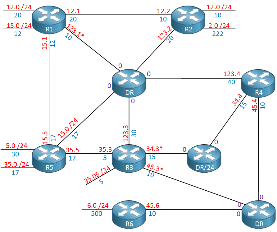
As a further exercise, I would encourage you to trace some OSPF path-costs using this new graph, and use the CLI to confirm your results. Inspect the routing table and LSDB for total path-costs as verification.
One point worthy of discussion is the point-to-multipoint network type. We learned all about DRs and how they make our shared segments more efficient. I am not going to discuss use cases for the P2MP network type as that is beyond the scope of this document.
However, configuring this network type will make a router form neighbors with any other router to which it can communicate; so, over a basic Ethernet segment, you would have N-1 neighbors, for a total of N*((N-1)/2) adjacencies. This could be a huge number in some cases. Let’s look at the effect of changing the network type from broadcast to P2MP on the 10.0.123.0/24 segment connecting R1, R2, R3, and R4.
First, let’s theorize what should happen.
- We should have one less LSA-2.
- We should have one less “Transit” link entry per router, since the network is no longer multi-access.
- We should have 4 new links per router. Three are point-to-point connections, and one is a stub network representing the local router’s endpoint (/32).
- So, in total, 1 less LSA, but 3 new links for R1, R2, R3, and R4.
For the sake of brevity, we will examine R1’s LSA-1 only.
R4#show ip ospf database router 1.1.1.1

            OSPF Router with ID (4.4.4.4) (Process ID 1)

		Router Link States (Area 0)

  LS age: 175
  Options: (No TOS-capability, DC)
  LS Type: Router Links
  Link State ID: 1.1.1.1
  Advertising Router: 1.1.1.1
  LS Seq Number: 8000000E
  Checksum: 0xDDC0
  Length: 120
  Number of Links: 8

    Link connected to: another Router (point-to-point)
     (Link ID) Neighboring Router ID: 3.3.3.3
     (Link Data) Router Interface address: 10.0.123.1
      Number of TOS metrics: 0
       TOS 0 Metrics: 10

    Link connected to: another Router (point-to-point)
     (Link ID) Neighboring Router ID: 4.4.4.4
     (Link Data) Router Interface address: 10.0.123.1
      Number of TOS metrics: 0
       TOS 0 Metrics: 10

    Link connected to: another Router (point-to-point)
     (Link ID) Neighboring Router ID: 2.2.2.2
     (Link Data) Router Interface address: 10.0.123.1
      Number of TOS metrics: 0
       TOS 0 Metrics: 10

    Link connected to: a Stub Network
     (Link ID) Network/subnet number: 10.0.123.1
     (Link Data) Network Mask: 255.255.255.255
      Number of TOS metrics: 0
       TOS 0 Metrics: 0

    Link connected to: another Router (point-to-point)
     (Link ID) Neighboring Router ID: 5.5.5.5
     (Link Data) Router Interface address: 10.0.15.1
      Number of TOS metrics: 0
       TOS 0 Metrics: 12

    Link connected to: a Stub Network
     (Link ID) Network/subnet number: 10.0.15.0
     (Link Data) Network Mask: 255.255.255.0
      Number of TOS metrics: 0
       TOS 0 Metrics: 12

    Link connected to: another Router (point-to-point)
     (Link ID) Neighboring Router ID: 2.2.2.2
     (Link Data) Router Interface address: 10.0.12.1
      Number of TOS metrics: 0
       TOS 0 Metrics: 20

    Link connected to: a Stub Network
     (Link ID) Network/subnet number: 10.0.12.0
     (Link Data) Network Mask: 255.255.255.0
      Number of TOS metrics: 0
       TOS 0 Metrics: 20
That’s quite a long list. The first 4 entries correspond with our new direct-connections to every router on the segment. Notice that P2MP does not have a network mask associated with it; other routers have no idea that this network is actually /24.
The P2MP network is represented as a collections of its endpoints only. Interesting that the corresponding stub network has no cost associated with it. Why? Because you can set per-neighbor costs with the P2MP network type, so the cost across each neighbor can be customized. But, the focus of this blog is graphs, so let’s view the final graph of this modification.
For those still new to this concept, I recommend you redraw the enter graph from scratch for extra practice. For clarity, I have omitted the costs from this graphic.
Well, it is certainly suboptimal and a bit sloppy, but it does not break any graph rules! We still have edges between exactly 2 vertices, except now we have removed the DR from the equation completely.
LSDB Optimizations
I will briefly discuss some techniques for optimizing the LSDB. Specifically, our goal would be to reduce extraneous routing information (reduce the “link count”) and to reduce vertices (LSA-2 in this case) from within the graph.
“Big O” notation is a way of measuring complexity in computer algorithms. Commonly we will measure algorithms as “orders of magnitude” rather than specific or exact complexity evaluations time, space, or both. For example, an algorithm that iterates over an array of N elements to search for a value would run in O(N) (pronounced “Order N”) time complexity. Likely, we would have a loop to iterate over the array and perform some action. Advanced searching algorithms like binary-sort work more intelligently and can run in O(log N) time, which is orders of magnitude better than O(N). This is not a computer science theory blog, so I will end this discussion now. Just understand that Big O notation is how we can compare algorithmic performance.
The modern Djikstra algorithm, which forms the basis of OSPF, runs in O(E + V log V) time complexity. We could improve the performance of the algorithm by reducing E (number of edges), V (number of vertices), or both. Even though we cannot change the algorithm by orders of magnitude, we can make small improvements. For routers that are CPU or memory constrained, this could be important.
Let’s begin with the easy one; reducing V. We already established that the number of vertices in the graph is the number of LSA1 plus LSA2. Removing LSA1 effectively means removing an entire router, which becomes more of a design issue than an optimization. Removing LSA2 though is quite simple; adjust the OSPF network type. We saw how this could be potentially devastating on large Ethernet segments, but using it on a multi-access network with only two routers reduces V by 1, improving the performance of SPF. Let’s look at a graph where the link between R3 and R4 was changed to “point-to-point”.
Well, we certainly reduced V by removing an unneeded DR, but in the process, we created two new edges (shown in orange for clarity). Examining the Big O notation, we see that both E and V are accounted for; reducing one at the cost of the other is something to be avoided if possible. Let’s take a look at R3 just to verify.
R3#show ip ospf database router self-originate

            OSPF Router with ID (3.3.3.3) (Process ID 1)

		Router Link States (Area 0)

  LS age: 11
  Options: (No TOS-capability, DC)
  LS Type: Router Links
  Link State ID: 3.3.3.3
  Advertising Router: 3.3.3.3
  LS Seq Number: 80000006
  Checksum: 0x67B0
  Length: 96
  Number of Links: 6

    Link connected to: a Transit Network
     (Link ID) Designated Router address: 10.0.45.3
     (Link Data) Router Interface address: 10.0.45.3
      Number of TOS metrics: 0
       TOS 0 Metrics: 10

    Link connected to: a Transit Network
     (Link ID) Designated Router address: 10.0.123.4
     (Link Data) Router Interface address: 10.0.123.3
      Number of TOS metrics: 0
       TOS 0 Metrics: 30

    Link connected to: another Router (point-to-point)
     (Link ID) Neighboring Router ID: 5.5.5.5
     (Link Data) Router Interface address: 10.0.35.3
      Number of TOS metrics: 0
       TOS 0 Metrics: 5

    Link connected to: a Stub Network
     (Link ID) Network/subnet number: 10.0.35.0
     (Link Data) Network Mask: 255.255.255.0
      Number of TOS metrics: 0
       TOS 0 Metrics: 5

    Link connected to: another Router (point-to-point)
     (Link ID) Neighboring Router ID: 4.4.4.4
     (Link Data) Router Interface address: 10.0.34.3
      Number of TOS metrics: 0
       TOS 0 Metrics: 15

    Link connected to: a Stub Network
     (Link ID) Network/subnet number: 10.0.34.0
     (Link Data) Network Mask: 255.255.255.0
      Number of TOS metrics: 0
       TOS 0 Metrics: 15
It looks like R3 has a sixth link now. Can we fix this? We can use “ip ospf prefix-suppression”, a rather obscure OSPF feature. Using this feature at the link level specifically tells OSPF “Do not create a corresponding stub network for this link” if the link is point-to-point or point-to-multipoint. The effect of this is that no one will have routing information for that interconnect between R3 and R4 … but in reality, does it matter? Imagine that it was simple a WAN link with no destination hosts on the segment. No one really needs a route to it, so in addition to optimizing OSPF for the entire area, we also save everyone a few bytes of memory by keeping the routing table smaller. I admit, this is totally insignificant on most modern routers, but for small, embedded systems where the router is comprised of a few chips, this matters.
After enabling prefix-suppression on R3’s link to R4, the graph is as follows:
That looks better, but R4 still has a stub network! We could easily clean that up by repeating the process on R4, and in most cases, we would. We would also do this on R1, R2, and R5 for their point-to-point links. Let’s verify R3 before going further.
R3#show ip ospf database router self-originate

            OSPF Router with ID (3.3.3.3) (Process ID 1)

		Router Link States (Area 0)

  LS age: 2
  Options: (No TOS-capability, DC)
  LS Type: Router Links
  Link State ID: 3.3.3.3
  Advertising Router: 3.3.3.3
  LS Seq Number: 80000007
  Checksum: 0xFA67
  Length: 84
  Number of Links: 5

    Link connected to: a Transit Network
     (Link ID) Designated Router address: 10.0.45.3
     (Link Data) Router Interface address: 10.0.45.3
      Number of TOS metrics: 0
       TOS 0 Metrics: 10

    Link connected to: a Transit Network
     (Link ID) Designated Router address: 10.0.123.4
     (Link Data) Router Interface address: 10.0.123.3
      Number of TOS metrics: 0
       TOS 0 Metrics: 30

    Link connected to: another Router (point-to-point)
     (Link ID) Neighboring Router ID: 5.5.5.5
     (Link Data) Router Interface address: 10.0.35.3
      Number of TOS metrics: 0
       TOS 0 Metrics: 5

    Link connected to: a Stub Network
     (Link ID) Network/subnet number: 10.0.35.0
     (Link Data) Network Mask: 255.255.255.0
      Number of TOS metrics: 0
       TOS 0 Metrics: 5

    Link connected to: another Router (point-to-point)
     (Link ID) Neighboring Router ID: 4.4.4.4
     (Link Data) Router Interface address: 10.0.34.3
      Number of TOS metrics: 0
       TOS 0 Metrics: 15
This looks better. We can also use this technique for advanced traffic engineering. For example, let’s assume that we actually had some hosts on the 34.0/24 subnet, but we wanted to force all traffic to those hosts through R4 and never through R3. Sure, we could mess with cost, but remember OSPF is always a bidirectional graph, and if R4 failed, R3 would become the gateway for those hosts. If this is undesirable, we can simply prevent R3 from advertising a stub link for that subnet, meaning no one could ever route traffic through R3 because R3 never claimed to be connected to that link. This gives us some additional intra-area filtering capability that is somewhat similar to the outbound distribute-list we find in non-link-state protocols.
One final comment on this feature; it can be enabled globally under the OSPF process as well using the command “prefix-suppression”. This ensures no routes are installed in the routing table, but only true stub links (those without neighbors). This would include loopbacks and local LAN segments. This is very handy in MPLS VPN environments where traffic transiting the MPLS core typically has at least 2 labels: an outer label (transport) and an inner label (VPN). The outer label just directs traffic between PEs, where the VPN labels determine to which specific customer (route, layer 2 circuit, etc) the traffic should be forwarded.
You may be thinking “How can a router not install a Transit network? After all, there is no stub-link to filter out.” Great question. OSPF will modify the network mask within the LSA-2 to signal to other routers that they should not install it in the routing table. It does so by setting the value to /32, which is bogus for any OSPF link with neighbors on it. As an example, we enable the feature under the OSPF process on R1 (or under the specific 10.0.123.0/24 interface on R1). Since R1 is the DR, it creates the LSA-2 for the segment. If we now look at R6, there is no reachability to this network anymore. Let’s verify the LSDB for the network mask change and also see what R6’s routing table says.
R6#show ip ospf database network 10.0.123.1

            OSPF Router with ID (6.6.6.6) (Process ID 1)

		Net Link States (Area 0)

  LS age: 49
  Options: (No TOS-capability, DC)
  LS Type: Network Links
  Link State ID: 10.0.123.1 (address of Designated Router)
  Advertising Router: 1.1.1.1
  LS Seq Number: 80000002
  Checksum: 0x4B33
  Length: 40
  Network Mask: /32
	Attached Router: 1.1.1.1
	Attached Router: 2.2.2.2
	Attached Router: 3.3.3.3
	Attached Router: 4.4.4.4
R6#show ip route 10.0.123.0
% Subnet not in tableI won’t go through every combination of configuration options, but hopefully you can see the optimization opportunities that prefix-suppression offers.
trying to change topology to speak via point-topoint over a switch. do u recommend any way to take a look at switche’s configuration
Hello Konstantinos
You can configure your OSPF network between two routers to be a point-to-point network type. More information about this can be found in the following lesson:
https://networklessons.com/ospf/ospf-point-to-point-network-type-over-frame-relay
Now the lesson describes such a network-type configuration over a Frame-Relay network. However, this can also be configured over ethernet links. And these ethernet links can be directly connected between routers, or they can indeed go over a switch.
Now, if the switch is a Layer 2 switch, it plays no pa
... Continue reading in our forum